Computation of Mathieu Functions with `MathieuFunctions.jl`

The Julia ecosystem has a package for computing Mathieu functions using the package implemented as MathieuFunctions.jl.

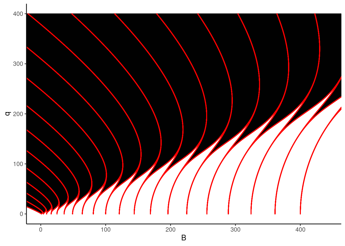
We will also learn how to record data in a DataFame and to save it to a CSV file (you could also use JSON or moder formats) to plot or analyse it using your program of choice (eg. R)

using MathieuFunctions
using DataFrames,CSV

df=DataFrame()
for q0 in 0:0.1:400
    for j=1:20
        dfaux=DataFrame(q=q0,
            A=charA(q0,k=j:j)[1],
            B=charB(q0,k=j:j)[1],
            kappa=j)
        append!(df,dfaux)
    end
end

#=
and we now simply save it to a CSV file
=#

CSV.write("./mathieu.csv", df)

For instance, we can now open an R session and plot this using ggplot. You can learn more about the lines which you can see in the article “Large scale radial stability density of Hill’s equation” by Broer, Levi and Simó.

library(ggplot2)
library(readr)


mathieu <- read_csv("mathieu.csv")

Rows: 80020 Columns: 4
── Column specification ────────────────────────────────────────────────────────
Delimiter: ","
dbl (4): q, A, B, kappa

ℹ Use `spec()` to retrieve the full column specification for this data.
ℹ Specify the column types or set `show_col_types = FALSE` to quiet this message.

  ggplot(mathieu,aes(x=B,xend=A,y=q,yend=q))+
  geom_segment(alpha=0.4)+theme_classic()+
  coord_fixed()+
  coord_cartesian(xlim=c(0,441))+
  geom_point(size=1e-5,color='red')+
    geom_point(aes(x=A),size=1e-5,color='red')

Coordinate system already present. Adding new coordinate system, which will
replace the existing one.

This page was generated using Literate.jl.

Computation of Mathieu Functions with MathieuFunctions.jl

Computation of Mathieu Functions with `MathieuFunctions.jl`