Introducing Ensemble Simulations: The Lorenz Equations

We have already seen the simulation of the trajectories of ODEs, as it would be the Lorenz equations:

using DifferentialEquations,Plots


function parameterized_lorenz!(du,u,p,t)
    x,y,z = u
    σ,ρ,β = p
    du[1] = dx = σ*(y-x)
    du[2] = dy = x*(ρ-z) - y
    du[3] = dz = x*y - β*z
end
u0 = [1.0,1.0,1.0] # Initial Conditions
tspan = (0.0,20)
p = [10.0,28.0,8/3]
f=ODEFunction(parameterized_lorenz!,syms = [:x, :y, :z])
prob = ODEProblem(f,u0,tspan,p)
sol = solve(prob)
plot(sol,idxs=:x)
savefig("lorenz_x.png")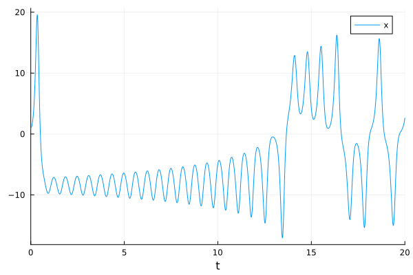

Lorenz simulation in \(x\)

When we want to simulate a bunch of solutions, called and ensemble simulation, we need to define a function which will assign new problems or initial conditions (one could also change the parameters) to the same ODEs.

A simple scenario is to modify the initial condition by a small random perturbation, to see the effect of dependence with respect to the initial conditions:

function prob_func(prob,i,repeat)
    @. prob.u0 = prob.u0+randn()*1e-2
    prob
end

The ensemble simulation is a set of and ODEProblem together with a function which updates the initial conditions or the parameters at every individual simulation.

ensemble_prob = EnsembleProblem(prob,prob_func=prob_func)

We now generate the simulation

sim = solve(ensemble_prob,trajectories=500)

and there is a plotting recipe to plot the simulation

plot(sim,idxs=(:x,:y),linealpha=0.1)
savefig("lorenz_ensemble_xy.png")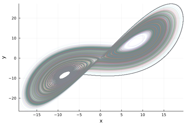

Ensemble simulation

We can analyze the solutions of our problem using quantiles and generate a plot

summ= EnsembleSummary(sim;quantiles=[0.05,0.95])
plot(summ,
    idxs=:x,
    fillalpha=0.2,
    ylims=(-20,20),
    background_color = RGB(0.2, 0.2, 0.2)
    )
savefig("lorenz_quantiles.png")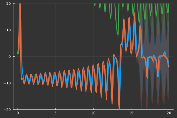

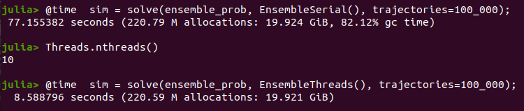
Ensemble Simulation Analysis

Using parallelism

An interesting feature of Ensemble Simulations is that one can use different kinds of parallelism or multithreading. From the documentation

- EnsembleSerial() - No parallelism
- EnsembleThreads() - The default. This uses multithreading. It's local (single computer, shared memory) parallelism only. Fastest when the trajectories are quick.
- EnsembleDistributed() - Uses pmap internally. It will use as many processors as you have Julia processes. To add more processes, use addprocs(n). See Julia's documentation for more details. Recommended for the case when each trajectory calculation isn't “too quick” (at least about a millisecond each?).
- EnsembleSplitThreads() - This uses threading on each process, splitting the problem into nprocs() even parts. This is for solving many quick trajectories on a multi-node machine. It's recommended you have one process on each node.
- EnsembleGPUArray() - Requires installing and using DiffEqGPU. This uses a GPU for computing the ensemble with hyperparallelism. It will automatically recompile your Julia functions to the GPU. A standard GPU sees a 5x performance increase over a 16 core Xeon CPU. However, there are limitations on what functions can auto-compile in this fashion, please see the DiffEqGPU README for more details

To start julia with multi-threading you need to run julia --threads=10 or any number of threads. No parallelism is equivalent to the serial version

@time  sim = solve(ensemble_prob, EnsembleSerial(), trajectories=10_000)

while a threaded version with the number of threads we called wen running julia is

@time  sim = solve(ensemble_prob, EnsembleThreads(), trajectories=10_000)

The improvement in time depend on your machine configuration. In my case, using 10 cores we get the following, which is above a factor of \(9\).

Parallelism in action