Discrete Maps using DifferentialEquations.jl

Hénon Map

The Hénon map is a classic example of a simple discrete dynamical system with an attractor which is neither a periodic point or a periodic orbit (or any other smooth invariant object) but a strange attractor. The equations are \[ x_{n+1}= 1-ax_n^2+y_n, \quad y_{n+1}=bx_n \] where \(a\) and \(b\) are parameters.

using DifferentialEquations,Plots

function henon_map!(u1,u,p=Float64[1.4,0.3],t=0)
    x,y= u
    a,b= p
    u1[1]=1-a*x^2+y
    u1[2]= b*x
    nothing
end
tspan = (0.0,10_000_000)
u=u0=Float64[1,1]
f=ODEFunction(henon_map!,syms = [:x, :y])
prob = DiscreteProblem(f,
    u0,tspan,Float64[1.4,0.3])
@time sol = solve(prob)


scatter(sol[100:10_000:end],
    idxs=(1,2),
    markersize=.01,
    alpha=0.1,
    legend=false)

savefig("./henon.png")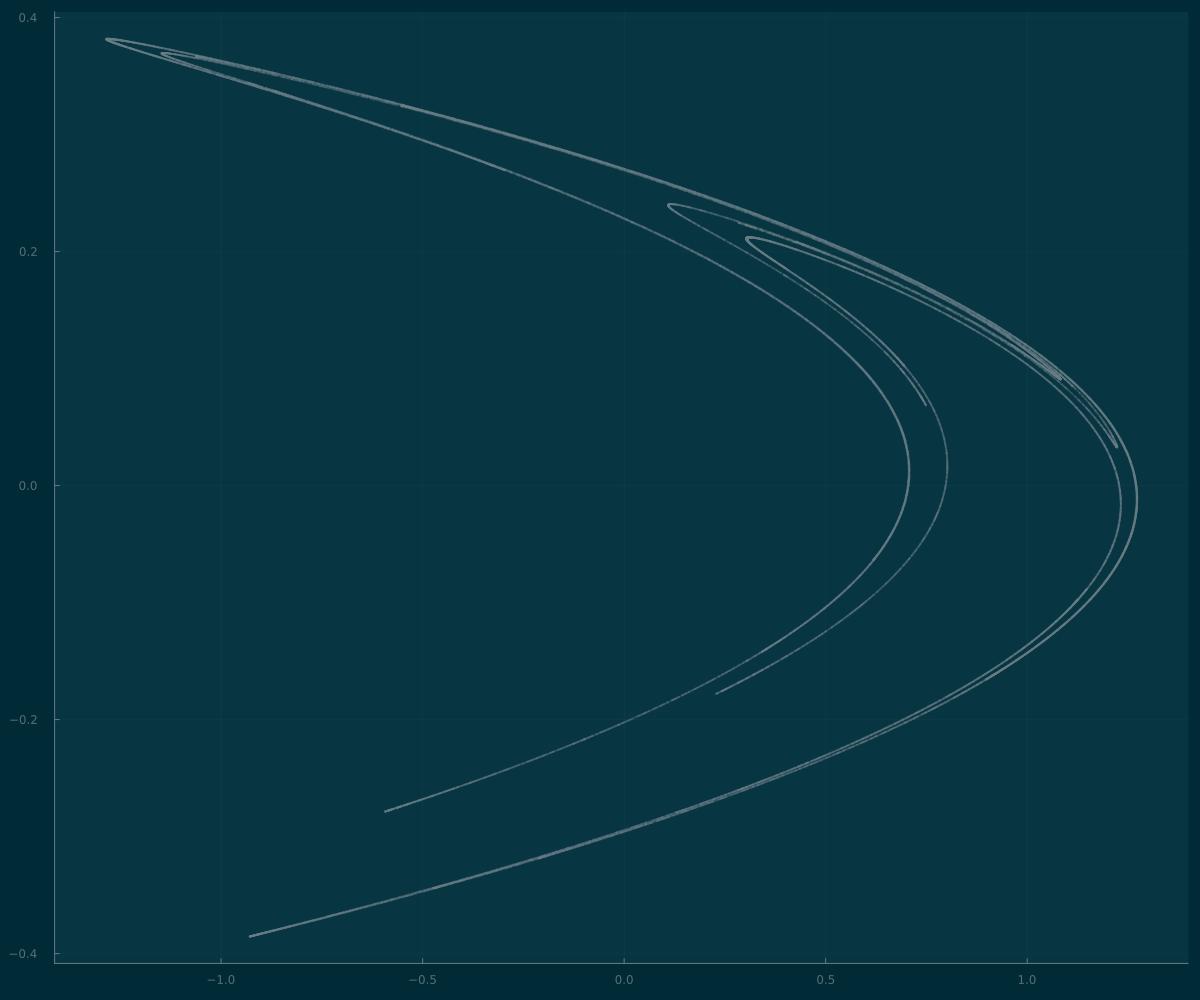

Hénon attractor as scatterplot

When plotting a large number of points, like this case, it is not very efficient because poitns are not going to plot many points in the same pixels. To obtain the visual effect of clustering of different passages at the same point we use alpha=0.1 for transparency.

To make the plot faster and more informative, we can simply plot a histogram2d:

histogram2d(sol[100:end],
    idxs=(1,2),
    bins=1000,
    legend=false)

savefig("henon_as_histogram.png")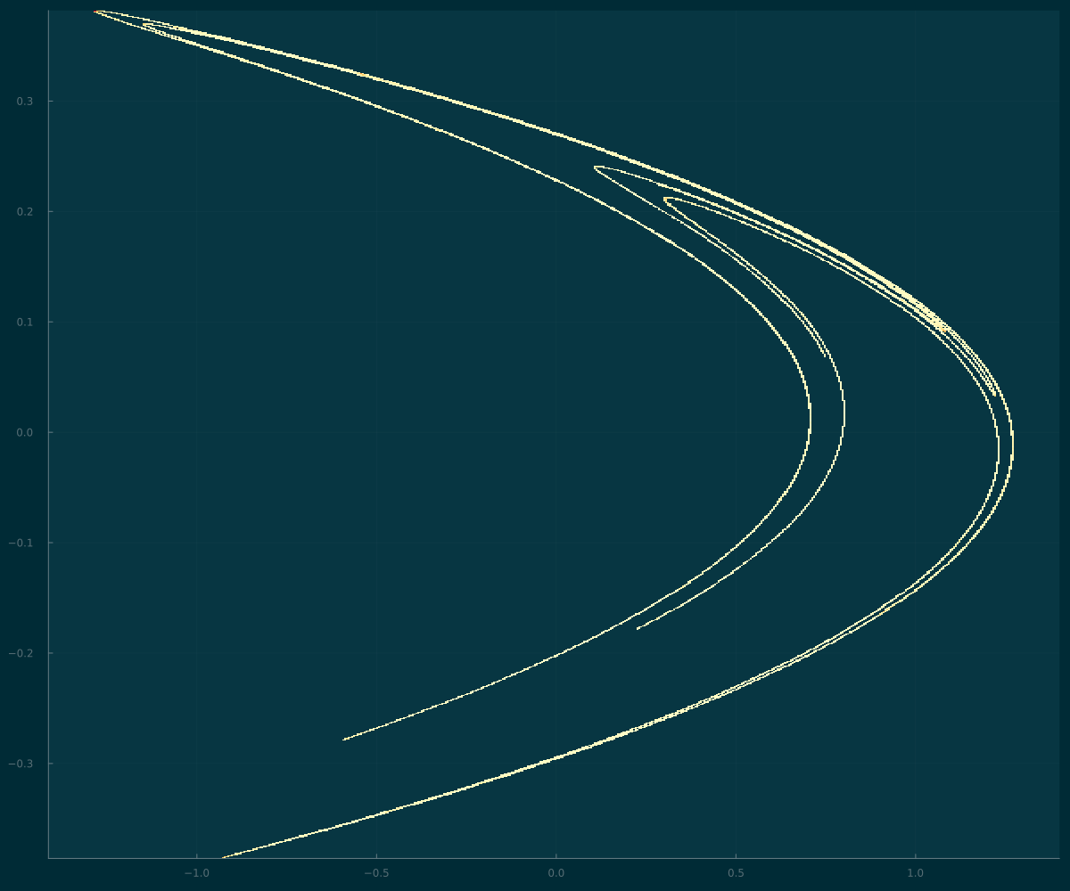

Hénon attractor as histogram2d

and now the colors represent the relative frequency that regions in the \((x,y)\) are visited by the orbits.

Finally, we export the dataset for further use

using DataFrames,CSV
df = DataFrame(sol)
CSV.write("./henon.csv",df)

so that we can also plot it with R

See also https://www.r-bloggers.com/2019/10/strange-attractors-an-r-experiment-about-maths-recursivity-and-creative-coding/

Extension: Clifford Attractors

Taken from https://fronkonstin.com/2017/11/07/drawing-10-million-points-with-ggplot-clifford-attractors/

Clifford attractors are a visually appealing example of strange attractors given by the iteration of a 2D system.

\[ x_{n+1}\, = \sin(a\, y_{n})\, +\, c\, \cos(a\, x_{n}) \]

\[ y_{n+1}\, = \sin(b\, x_{n})\, +\, d\, \cos(b\, y_{n}) \]

where \(a,b,c\) and \(d\) are different parameters. A choice of parameters is

a=-1.24458046630025 b=-1.25191834103316 c=-1.81590817030519 d=-1.90866735205054

Let us produce the plot:

using DifferentialEquations

function clifford_map!(u1,u,p,t=0)
    x,y= u
    a,b,c,d= p
    u1[1]=sin(a*y)+c*cos(a*x)
    u1[2]= sin(b*x)+d*cos(b*y)
    nothing
end

tspan = (0.0,100_000)
u=u0=Float64[0,0]
p0=Float64[-1.24458046630025,
    -1.25191834103316,
    -1.81590817030519,
    -1.90866735205054]

f=ODEFunction(clifford_map!,syms = [:x, :y])
prob = DiscreteProblem(f,
    u0,tspan,p0)
@time sol = solve(prob)


scatter(sol[100:end],
    idxs=(1,2),
    markersize=.01,
    alpha=0.1,
    legend=false,
    size = (1200, 1000))

savefig("./clifford.png")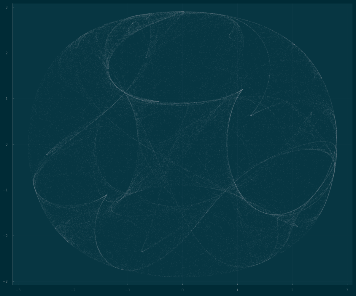

Clifford attractor as scatterplot

histogram2d(sol[100:end],
    idxs=(1,2),
    bins=2000,
    legend=false,
    size = (1200, 1000))

savefig("./clifford_as_histogram.png")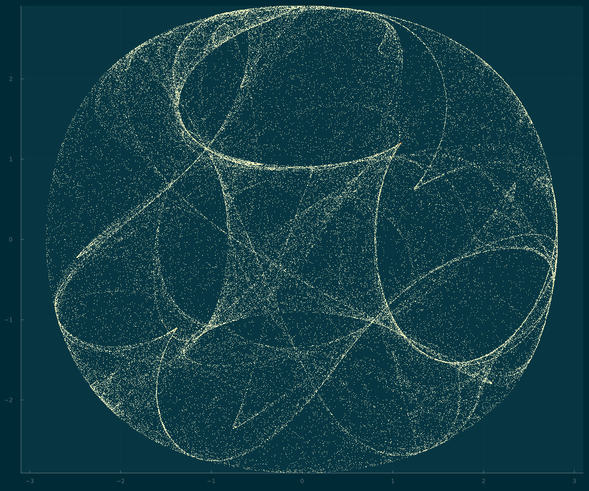

Clifford attractor plotted as a histogram2d

We finally save it as a csv file for later use

using DataFrames,CSV
df = DataFrame(sol)
CSV.write("./clifford.csv",df)